We want to find a close upper bound on the contribution ![]() of
each task
of
each task ![]() to the demand in a particular window of time. We
have bounded the contribution to
to the demand in a particular window of time. We
have bounded the contribution to ![]() of the head of the window. We
are now ready to derive a bound on the whole of
of the head of the window. We
are now ready to derive a bound on the whole of ![]() , including
the contributions of head, body, and tail for the EDF case.
, including
the contributions of head, body, and tail for the EDF case.
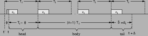
The tail of a window with respect to a task ![]() is the
final segment, beginning with the release time of the carried-out
job of
is the
final segment, beginning with the release time of the carried-out
job of ![]() in the window (if any). The carried-out job has
a release time within the window and its next
release time is beyond the window. That is, if the release time of the
carried-out job is
in the window (if any). The carried-out job has
a release time within the window and its next
release time is beyond the window. That is, if the release time of the
carried-out job is ![]() ,
,
![]() . If there is no
such job, then the tail of the window is null. We use the symbol
. If there is no
such job, then the tail of the window is null. We use the symbol
![]() to denote the length of the tail, as shown in
Figure 2.
to denote the length of the tail, as shown in
Figure 2.
The body is the middle segment of the window, i.e., the portion that is not in the head or the tail. Like the head and the tail, the body may be null (provided the head and tail are not also null).
Unlike the contribution of the head, the contributions of the body and tail
to ![]() do not depend on the schedule leading up to the window. They
depend only on the release times within the window,
which in turn are constrained by the period
do not depend on the schedule leading up to the window. They
depend only on the release times within the window,
which in turn are constrained by the period
![]() and by the release time of the carried-in job of
and by the release time of the carried-in job of
![]() (if any).
(if any).
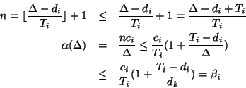
Let ![]() be the number of jobs of
be the number of jobs of ![]() released in the body and tail.
If both body and tail are null,
released in the body and tail.
If both body and tail are null,
![]() ,
, ![]() , and
the contribution of the body and tail is zero.
Otherwise, the body and or the tail is non-null, the combined length of the
body and tail is
, and
the contribution of the body and tail is zero.
Otherwise, the body and or the tail is non-null, the combined length of the
body and tail is
![]() , and
, and ![]() .
.
Proof:
We will identify a worst-case situation, where ![]() achieves the
largest possible value for a given value of
achieves the
largest possible value for a given value of ![]() . For
simplicity, we will risk overbounding
. For
simplicity, we will risk overbounding ![]() by considering a wide
range of possibilities, which might include some cases that would
not occur in a specific busy window.
We will start out by looking only at the case where
by considering a wide
range of possibilities, which might include some cases that would
not occur in a specific busy window.
We will start out by looking only at the case where
![]() ,
then go back and consider later the case where
,
then go back and consider later the case where ![]() .
.
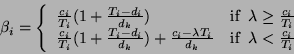
Looking at Figure 4, it is easy to see that the
maximum possible contribution of the body and tail to ![]() is
achieved when successive jobs are released as close together as
possible. Moreover, if one imagines shifting all the release
times in Figure 4 earlier or later, as a block,
one can see that the maximum is achieved when the last job is
released just in time to have its deadline coincide with the end
of the window. That is, the maximum contribution to
is
achieved when successive jobs are released as close together as
possible. Moreover, if one imagines shifting all the release
times in Figure 4 earlier or later, as a block,
one can see that the maximum is achieved when the last job is
released just in time to have its deadline coincide with the end
of the window. That is, the maximum contribution to ![]() from the
body and tail is achieved when
from the
body and tail is achieved when ![]() . In this case there
is a tail of length
. In this case there
is a tail of length ![]() and the number of complete executions of
and the number of complete executions of
![]() in the body and tail is
in the body and tail is
![]() .
.
From Lemma 9, we can see that the contribution
![]() of the head to
of the head to ![]() is a nonincreasing function of
is a nonincreasing function of ![]() .
Therefore,
.
Therefore, ![]() is maximized when
is maximized when ![]() is as small as
possible. However, reducing
is as small as
possible. However, reducing ![]() increases the size of the head,
and may reduce the contribution to
increases the size of the head,
and may reduce the contribution to ![]() of the body and tail.
of the body and tail.
Looking at Figure 4, we see that the
length of the head, ![]() , cannot be
larger than
, cannot be
larger than
![]() without pushing all of the final
execution of
without pushing all of the final
execution of ![]() outside the window. Reducing
outside the window. Reducing ![]() below
below
![]() results in at most a linear
increase in the contribution of the head, accompanied by a
decrease of
results in at most a linear
increase in the contribution of the head, accompanied by a
decrease of ![]() in the contribution of the body and tail.
Therefore the value of
in the contribution of the body and tail.
Therefore the value of ![]() is maximized
for
is maximized
for
![]() .
.
We have shown that
It is now time to consider the case where ![]() .
There can be no body or tail contribution, since it is
impossible for a job of
.
There can be no body or tail contribution, since it is
impossible for a job of ![]() to have both release time and
deadline within the window. If
to have both release time and
deadline within the window. If ![]() is nonzero, the only
contribution can come from a carried-in job. Lemma 9
guarantees that this contribution is at most
is nonzero, the only
contribution can come from a carried-in job. Lemma 9
guarantees that this contribution is at most
![]() ,
,
For
![]() we have
we have
Proof:
The objective of the proof is to find an upper bound for ![]() that is independent of
that is independent of ![]() .
Lemma 10 says that
.
Lemma 10 says that
There are two cases:
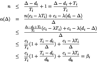
Case 1:
![]() .
.
We have
![]() , and
, and
![]() .
Since we also know that
.
Since we also know that ![]() , we have
, we have
![]() .
From the definition of
.
From the definition of ![]() , we have
, we have
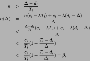
Case 2:
![]() .
.
We have
![]() . Since
. Since
![]() ,
,
We have two subcases, depending on the sign of
![]() .
.
Case 2.1:
![]() . That is,
. That is,
![]() .
.
From the definition of ![]() , it follows that
, it follows that
Case 2.2:
![]() . That is,
. That is,
![]() .
.
From the definition of ![]() , it follows that
, it follows that
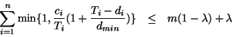
![]()
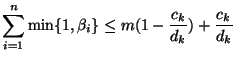
Using the above lemmas, we can prove the following theorem, which provides a sufficient condition for schedulability.
Proof: The proof is by contradiction. Suppose some task misses a deadline. We will show that this leads to a contradiction of (1).
Let ![]() be the first
task to miss a deadline and
be the first
task to miss a deadline and ![]() be a busy window for
be a busy window for
![]() , as in Lemma 7.
Since
, as in Lemma 7.
Since ![]() is
is
![]() -busy
we have
-busy
we have
![]() . By
Lemma 11,
. By
Lemma 11,
![]() , for
, for
![]() .
Since
.
Since ![]() is the first missed deadline, we know that
is the first missed deadline, we know that
![]() .
It follows that
.
It follows that
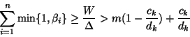
The schedulability test above must be checked individually for
each task ![]() . If we are willing to sacrifice some precision,
there is a simpler test that only needs to be checked once for
the entire system of tasks.
. If we are willing to sacrifice some precision,
there is a simpler test that only needs to be checked once for
the entire system of tasks.
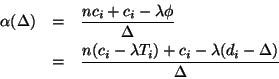
Sketch of proof:
Corollary 13 is proved by repeating the proof of
Theorem 12, adapted to fit the definitions of ![]() and
and ![]() .
.
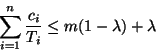
![]()
Goossens, Funk, and Baruah[8] showed the following:
Their proof is derived from a theorem in [7], on
scheduling for uniform multiprocessors, which in turn is
based on [16]. This can be shown independently as
special case of Corollary 13,
by replacing ![]() by
by ![]() .
.
The above cited theorem of Goossens, Funk, and Baruah is
a generalization of a result of Srinivasan and Baruah[18],
who defined a periodic task set
![]() to
be a light system on
to
be a light system on ![]() processors if it satisfies the
following properties:
processors if it satisfies the
following properties:
They then proved the following theorem.
The above result is a special case of Corollary 14,
taking
![]() .
.