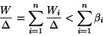
We now try to derive an upper bound on the load of a window
leading up to a missed deadline.
If we can find such an upper bound
![]() it will follow from Lemma 3 that
the condition
it will follow from Lemma 3 that
the condition
![]() is
sufficient to guarantee schedulability.
The upper bound
is
sufficient to guarantee schedulability.
The upper bound ![]() on
on ![]() is the sum of individual
upper bounds
is the sum of individual
upper bounds ![]() on the load
on the load
![]() due to each individual task
in the window. It then
follows that
due to each individual task
in the window. It then
follows that
While our first interest is in a problem window, it turns out that
one can obtain a tighter schedulability condition by considering a
well chosen downward extension
![]() of a problem
window, which we call a window of interest.
of a problem
window, which we call a window of interest.
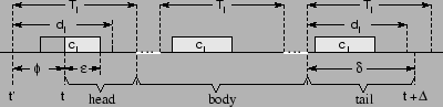
For any task ![]() that can execute in a window of interest,
we divide the window into three parts, which we call the head,
the body, and the tail of the window with respect to
that can execute in a window of interest,
we divide the window into three parts, which we call the head,
the body, and the tail of the window with respect to
![]() , as shown in Figure 2. The
contribution
, as shown in Figure 2. The
contribution ![]() of
of ![]() to the demand in the window of
interest is the sum of the contributions of the head, the body,
and the tail. To obtain an upper bound on
to the demand in the window of
interest is the sum of the contributions of the head, the body,
and the tail. To obtain an upper bound on ![]() we look at each
of these contributions, starting with the head.
we look at each
of these contributions, starting with the head.
The head is the initial segment of the window up to the
earliest possible release time (if any) of ![]() within or
beyond the beginning of the window. More precisely, the head of
the window is the interval
within or
beyond the beginning of the window. More precisely, the head of
the window is the interval
![]() ,
such that there is a job of task
,
such that there is a job of task ![]() that is released at time
that is released at time
![]() ,
,
![]() ,
, ![]() . We call such a
job, if one exists, the carried-in job of the window with
respect to
. We call such a
job, if one exists, the carried-in job of the window with
respect to ![]() . The rest of the window is the body and tail,
which are formally defined closer to where they are used, in
Section 5.
. The rest of the window is the body and tail,
which are formally defined closer to where they are used, in
Section 5.
Figure 2 shows a window with a carried-in job.
The release time of the carried-in job is ![]() , where
, where
![]() is the offset of the release time from the beginning of the
window. If the minimum interrelease time constraint prevents any
releases of
is the offset of the release time from the beginning of the
window. If the minimum interrelease time constraint prevents any
releases of ![]() within the window, the head comprises the
entire window. Otherwise, the head is an initial segment of the
window. If there is no carried-in job, the head is said to be
null.
within the window, the head comprises the
entire window. Otherwise, the head is an initial segment of the
window. If there is no carried-in job, the head is said to be
null.
The carried-in job has two impacts on the demand in the window:
If there is a carried-in job, the contribution of the head to ![]() is
the residual compute time of the carried-in job at the beginning of
the window, which we call the carry-in. If there is no
carried-in job, the head makes no contribution to
is
the residual compute time of the carried-in job at the beginning of
the window, which we call the carry-in. If there is no
carried-in job, the head makes no contribution to ![]() .
.
The carry-in of a job depends on the competing demand.
The larger the value of ![]() the longer is the time
available to complete the carried-in job before the beginning of
the window, and the smaller should be the value of
the longer is the time
available to complete the carried-in job before the beginning of
the window, and the smaller should be the value of ![]() . We
make this reasoning more precise in Lemmas 5 and
9.
. We
make this reasoning more precise in Lemmas 5 and
9.
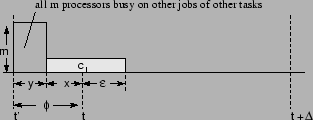
Proof:
Suppose ![]() has nonzero carry-in. Let
has nonzero carry-in. Let ![]() be the amount of time
that
be the amount of time
that ![]() executes in the interval
executes in the interval ![]() . For example,
see Figure 3. By definition,
. For example,
see Figure 3. By definition,
![]() .
Since the job of
.
Since the job of ![]() does not complete in the interval,
whenever
does not complete in the interval,
whenever ![]() is not executing during the interval all
is not executing during the interval all ![]() processors must be executing other jobs that can preempt that job of
processors must be executing other jobs that can preempt that job of
![]() . This has two consequences:
. This has two consequences:
From the first observation above, we have
![]() .
Putting these two facts together gives
.
Putting these two facts together gives
Since the size of the carry-in, ![]() , of a given task depends
on the specific window and on the schedule leading up to the beginning
of the window, it seems that bounding
, of a given task depends
on the specific window and on the schedule leading up to the beginning
of the window, it seems that bounding ![]() closely depends on
being able to restrict the window of interest.
Previous analysis of single-processor schedulability (e.g., [13,3,10,11]) bounded carry-in to zero by considering the busy
interval leading up to a missed deadline, i.e., the interval
between the first time
closely depends on
being able to restrict the window of interest.
Previous analysis of single-processor schedulability (e.g., [13,3,10,11]) bounded carry-in to zero by considering the busy
interval leading up to a missed deadline, i.e., the interval
between the first time ![]() at which a task
at which a task ![]() misses a deadline
and the last time before
misses a deadline
and the last time before ![]() at which there are no pending jobs
that can preempt
at which there are no pending jobs
that can preempt ![]() . By definition, no demand
that can compete with
. By definition, no demand
that can compete with ![]() is carried into the busy
interval. By modifying the definition of busy interval slightly, we
can also apply it here.
is carried into the busy
interval. By modifying the definition of busy interval slightly, we
can also apply it here.
Proof:
Let ![]() be any problem window for
be any problem window for ![]() . By
Lemma 3 the problem window is
. By
Lemma 3 the problem window is ![]() -busy, so
the set of
-busy, so
the set of ![]() -busy downward extensions of the problem window is
non-empty. The system has some start time, before which no task is
released, so the set of all
-busy downward extensions of the problem window is
non-empty. The system has some start time, before which no task is
released, so the set of all ![]() -busy downward extensions of the problem
window is finite. The set is totally ordered by length.
Therefore, it has a unique maximal element.
-busy downward extensions of the problem
window is finite. The set is totally ordered by length.
Therefore, it has a unique maximal element. ![]()
Observe that a busy window for ![]() contains a problem window for
contains a problem window for
![]() , and so
, and so
![]() .
.
Proof:
The proof follows from Lemma 5 and the definition
of ![]() -busy.
-busy. ![]()