|
COT 4401 Top 10 Algorithms Chris Lacher Graph Search |
| index↑ |
|
|
COT 4401 Top 10 Algorithms Chris Lacher Graph Search |
| index↑ |
We have looked at BFS and DFS in graphs. It is possible to phrase these as very similar code with very different outcomes, as in the Graphs1 notes. Here is the algorithm DFSearch(v), using a double-ended control queue conQ:
class DFSurvey
{
public:

  typedef uint32_t Vertex;

         DFSurvey ( const Graph& g );
  void   Search   ( );
  void   Search   ( Vertex v );
  void   Reset    ( );

  Vector < unsigned >  dtime;   // discovery time
  Vector < unsigned >  ftime;   // finishing time
  Vector < Vertex >    parent;  // parent in DFS tree
  Vector < Color >     color;   // state of vertex at any point during search/survey

private:
  unsigned          time_;
  const Graph&      g_;
  Vector < bool >   visited_ ;
  Deque  < Vertex > conQ_  ;
};
The class contains a reference to a graph object on which the survey is performed, private data used in the algorithm control, and public variables to house four results of the survey - discovery time, finishing time, parent, and color for each vertex in the graph. (These could be privatized with accessors and other trimmings for data security.) These data are instantiated by the survey and have the following interpretation when the survey is completed:
code description dtime[x] time of discovery of vertex v ftime[x] time of finishing processing vertex v parent[x] the parent in the search tree - the vertex from which x was discovered color[x] white, grey, or black: white = undiscovered, grey = being processed, black = finished
During the course of Search(), vertices are colored gray at discovery time and pushed onto the control queue in LIFO order, and colored black at finishing time and popped from the queue. At any given time during Search(), the gray vertices are precisely those in the LIFO control queue. The Search(v) method is DFSearch(v) with the pre- and post-processing functions defined to maintain the survey data. Note however that the visited flags are not automatically unset at the start, so that the method can be called more than once to continue the survey in any parts of the graph that were not reachable from v. Global time is incremented immediately after each use, which ensures that no two time stamps are the same.
void DFSurvey::Search( Vertex v )
{
  dtime[v] = time_++;
  conQ_.Push(v);
  visited_[v] = true;
  color[v]    = grey;
  while (!conQ_.Empty())
  {
    f = conQ_.Front();
    if (n = unvisited adjacent from f in g_)
    {
      dtime[n] = time_++;
      conQ_.PushFront(n);  // PushLIFO
      visited_[n] = true;
      parent[n]   = &f;
      color[n]    = grey;
    }
    else
    {
      conQ_.PopFront();
      color[f] = black;
      ftime[f] = time_++;
    }
  }
}
The no-argument Search method repeatedly calls Search(v), thus ensuring that the survey considers the entire graph.
void DFSurvey::Search()
{
  Reset();
  for (each vertex v of g_)
  {
    if (color[v] == white) Search(v);
  }
}
void DFSurvey::Reset()
{
  for (each vertex v of g_)
  {
    visited_[v] = 0;
    parent[v] = null;
    color[v] = white;
    dtime[v] = 2|V|;  // last time stamp is 2|V| -1
    ftime[v] = 2|V|;
    time_ = 0;
  }
}
Note that the only places where BFS and DFS differ is in the way vertices are inserted into the double-ended control queue. DFS (shown above) pushes at the front and BFS pushes at the back. We always Pop at the front of conQ, so DFS exhibits abstract Stack/LIFO behavior and BFS exhibits abstract Queue/FIFO behavior.
We can generalize this graph search algorithm by using a priority queue for conQ. This is a class of algorithms known generally as Best First Search, the beginning of "intelligent" search.
Algorithm A* was introduced by Peter Hart, Nils Nilsson and Bertram Raphael in 1968. It has been in heavy use ever since in both research and practical applications. There is at least one web site maintained specifically to explain algorithm A* and keep up with its evolving applications and descendants, which include many uses in navigation systems, AI, and electronic games.
Algorithm A* uses two notions of distance between vertices x, y in a weighted graph: actual (path) distance and heuristic distance, defined by a distance estimator heuristic. Let D(x,y) denote the path distance from x to y, that is, the weight of a shortest path from x to y, where path weight is defined to be the total weight of the path, and assume we have a heuristic distance estimator H(x,y). We will further assume that the heuristic function H satisfies both of the following properties:
That is, H never over-estimates distances and H obeys a "triangle inequality". (We use the notation of directed edges, but the context can be either directed or undirected.)
Lemma (Admissibility). If H is monotonic and H(x,x) = 0 for all x then H is admissible.
Proof. Let P = {x, v1, v2, . . . , vk-1, y} be a shortest path from x to y. Then
H(x,y) <= w(x,v1) + H(v1,y) // applying monotonic property at v1 <= w(x,v1) + w(v1,v2) + H(v2,y) // applying monotonic property at v2 <= w(x,v1) + w(v1,v2) + w(v2,v3) + H(v3,y) // applying monotonic property at v3 . . . <= w(x,v1) + w(v1,v2) + . . . + w(vk-1,y) + H(y,y) // applying monotonic property at vk-1 == w(x,v1) + w(v1,v2) + . . . + w(vk-1,y) // applying H(y,y) = 0
That is, H(x,y) is no greater than the total weight of the (minimal weight) path from x to y, which is by definition D(x,y). QED
We now set up the notation for Algorithm A* as it is traditionally done: Suppose start is a start vertex and goal is a goal vertex, and define
g(x) = D(start,x) = path distance from start to x h(x) = H(x,goal) = path distance from x goal f(x) = g(x) + h(x) = A* search priority at x
We will use the following example to motivate and illustrate algorithm A*: The graph represents a roadmap, with vertices being cities or other road intersections and edges being road segments directly connecting two vertices. The distances are w(x,y) = the weight (length) of the road segment directly connecting x to y; D(x,y) = the shortest roadway distance from x to y; and H(x,y) = the straight-line (euclidean) distance between x and y. We have a start city start and a destination city goal and wish to calculate the driving distance from start to goal.
A* sets up as follows:
vertex x city edge e = (x,y) road between cities x and y w(e) length of road between x and y g(x) D(start,x) = shortest road distance from start to x h(x) H(x,goal) = straight-line distance from x to goal f(x) g(x) + h(x) = D(start,x) + H(x,goal)
The euclidian distance function is admissible and monotonic, so our assumptions are met by the example. Note in passing that H(x,y) is easily calculated directly from GPS data and w(e) is available from a database of road segment lengths. D(x,y) can be calculated using A* but is not readily available.
Algorithm A* uses the same search pattern as that of Prim and Dijkstra, using f(x) as priority in the queue. The queue strategy can be either profligate or frugal. (See [Lacher, Graphs2].) The queue is called the OPEN set in the following statement of the algorithm. The CLOSED set consists of the black vertices with which the algorithm is finished. The white vertices have not yet been encountered.
Algorithm A*
find a shortest path from start to goal

Uses:   ordered set OPEN of vertices, ordered by F
        cost functions G, H, F = G + H

OPEN   = set of gray vertices
CLOSED = set of black vertices

initialize visited[x] = 0, parent[x] = NULL, color[x] = white

visited[start] = 1;
parent[start]  = NULL;
color[start]   = gray;
OPEN.Insert(start,F(start));

while (!q.Empty())
{
  f = q.Front();
  if (f == goal) break;
  for each adjacent n from f
  {
    cost = G(f) + w(f,n);
    if (color[n] = white)
    {
      G(n) = cost;
      F(n) = cost + H(n);
      parent[n] = f;
      OPEN.Insert(n,F(n));
    }
    else if (color[n] = gray)
    {
      if (cost < G(n)) // path through n is not optimal
      { // Relax
        G(n) = cost;
        F(n) = cost + H(n);
        parent[n] = f;
        OPEN.DecreaseKey(n, F(n));
      }
    }
    else // color[n] = black
    {
      // no action needed when H is admissable and monotonic
      // otherwise it is possible n needs to be reconsidered
    }
  }
  OPEN.Remove(f);
  color[f] = black;
}
reconstruct reverse path from goal to start by following parent pointers
Theorem (Correctness of A*). Using an admissible monotonic heuristic, if there is a path from start to goal, A* will always find one with minimum weight.
The proof is similar to that of the Dijkstra SSSP. This is good news: it means that even if our "intelligent" heuristic makes a lot of bad choices, worse than random, we will still muddle through. Of course: (1) If the heuristic is "good" we will find the goal sooner than the "random" choices made by DFS or BFS; and (2) If the heuristic is bad, it may take longer. Choose heuristics carefully.
In the example used above, the heuristic is an actual distance (in that instance, the Euclidian straight-line distance in a plane, or, more accurately, the great circle distance on a globe). It turns out that Algotithm A* converges even in the case that the heuristic estimator is not monotonic, and this is an important category of applications. In areas such as fictional worlds where there was never a Euclid (applications in electronic games), or in non-geometric applications such as knowledge domains (applications in AI), the heuristic may not satisfy the "triangle inequality" yet still be an intuitively justifiable estimate of distance in the associated graph or digraph.
For the remainder of this chapter (including the exercises) assume that the search graph is the isomorph of a rectangular array of square cells. Thus in particular the edge weights are all 1.00. Also consider three algorithms for finding a shortest path from start to goal:
In other words, we re-phrase the first two as point-to-point path algorithms rather than complete searches. This puts the three processes on the same footing for comparison.
Exercise 1. In the context of mazes, explain the differences, if any, between BFS(start,goal) and Dijkstra(start,goal).
Demo by Chad Duncan
Note that in the demo above, you can create a "maze" by inserting blocking cells into the blank canvas.
Exercise 2.
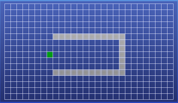
Begin with the following maze and start position:
Place the goal cell on the opposite side of the North-South wall from the start cell. Show the discovered (non-white) cells after applying each of the three algorithms. (Assume that adjacency lists order cells North, East, South, West.) You can use different color/notation on one image or submit different images.)
Exercise 3. Explain what the effect of a call to Shuffle has on BFS, Dijkstra, and A*.
| index↑ |