Rate Monotone Scheduling

These notes make use of mathematical symbols that may not be visible with the default settings on some versions of some browsers.

If a blank space appears to the left of any of the names in the table above, or the symbol looks strange, try changing the font settings on your browser or using a different browser.

Context

This analysis is based on the following assumptions:

• all tasks are periodic
• all tasks are independent
• relative deadline ≤ period
• scheduling policy is preemptive deadline-monotonic fixed-priority
  i.e., jobs with shorter relative deadline have higher priority
  • priority is static w.r.t. both jobs and tasks

Rate Monotonic vs. Deadline-Monotonic Scheduling

Rate Monotone (RM)

shorter period (higher rate) ⇒ higher priority

Deadline Monotone (DM)

shorter relative deadline ⇒ higher priority

The original paper on this topic, by Liu & Layland, coined the term Rate Monotone scheduling, but made the assumption that the relative deadline of each task is the same as its period. Under that condition, RM and DM scheduling are equivalent. Later research pointed out relaxed the assumption that relative dealine equal period, and showed that what really matters is the relative deadline.

People still sometimes use the terms "Rate Monotone" and "Rate Monotonic" (RM) loosely, to include both RM and DM scheduling, since most of the results for RM scheduling have been shown to also apply to DM scheduling.

Optimality of RM and DM Scheduling for Harmonic Tasks

Theorem: A system of simply periodic, independent, preemptable tasks whose relative deadlines are not smaller than their periods is schedulable on one processor according to the RM algorithm if and only if its total utilization is less than or equal to one.

Here, a system of tasks is simply periodic if for every pair of tasks such that T_i < T_k, T_k is an integer multiple of p_i. Such a system is sometimes said to be harmonic.

Optimality of DM Scheduling in the General Case

Theorem 6.4 (J. Liu): A system of periodic independent preemptable tasks that are in phase and whose relative deadlines are less than or equal to their periods is schedulable on one processor according to the DM algorithm whenever it can be scheduled according to any fixed-priority algorithm.

J. Liu leaves the crucial part of the proof of this theorem as an exercise for the reader. It is probably a good thing for you do do that exercise.

The in-phase restriction can later be dropped, using the critical instant theorem.

Notation::

In the original L&Lpaper, τ_i is the name of a task, T_i is the task's period, and C_i is the task's compute (execution) time. We use that notation for the following.

Critical Instants - Original L & L Definitions and Theorem

A critical instant for a task is defined to be an instant at which a request for that task will have the largest response time

A critical time zone for a task is the time interval between a critical instant and the end of the reponse to the corresponding request of the task.

Theorem: A critical instant for any task occurs whenever the task is requested simultaneously with requests for all higher priority tasks.

The definitions and theorem above are stated in the words of L & L. They may seem rather imprecise. More precise definitions will be given later.

Original L & L Proof

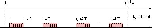
Proof: Let τ₁, τ₂, ... τ_m denote a set of priority-ordered tasks with τ_m being the task with the lowest priority. Consider a particular request for τ_m that occurs at time t₁. Suppose that between t₁ and t₁+T_m, the time at which the subsequent request of τ_m occurs, requests for task τ_i , i < m, occur at t_i, t_i+T_i, ... t_i+kT_i , as illustrated in Figure 1.

Clearly, the preemption of τ_m by τ_i will cause a certain amount of delay in the completion of the request for τ_m that occurred at t₁, unless the request for τ_m is completed before t_i.

Moreover, from the figure above we see immediately that advancing the request time t₂ will not speed up the completion of τ_m. The completion time of τ_m is either unchanged or delayed by such advancement. Consequently, the delay in the completion of τ_m is largest when t₂ coincides with t₁.

Repeating the argument for all τ_k, k = 2, ... m-1, we prove the theorem.

The diagram, notation, and wording are exactly as in the published paper. In particular, the notation C_i is used for execution time and T_i is used for the period of task τ_i.

Need to Consider Full Busy Interval

The statement that we are supposed to see immediately above is not so obviously true, as the example below illustrates. Consider the following task set.

The diagram below illustrates how advancing the request time t₂ to t₁ will speed up the completion of t₃ (unless we also simultaneously move up the request time of t₁).

To avoid this fallacy, we need to look at a longer interval, which we call the busy interval leading up to the critical instant.

Refined Definition of Critical Instant

A critical instant of a task τ_i is a time instant t (in a particular schedule for a task set containing τ_i) such that

• the job in τ_i released at time t has the maximum response time of all jobs in τ_i (over all schedules of the given task set), if such a maximum exists.
• the response time of the job τ_i exceeds D_i, if the response time of τ_i is unbounded (over all schedules).

Refined Critical Instant Theorem

Theorem 6.5: In a fixed priority (preemptive) scheduling system where every job completes before the next job in the same task is released, a critical instant of any task τ_i occurs when one of its jobs J_i,c is released at the same time with a job in every higher priority task, i.e., r_i,c = r_k,x for some x for each k = 1, 2, ... i-1.

The Critical Instant Theorem is sometimes called the Critical Zone Theorem.

A consequence of this theorem is that RM/DM scheduling is optimal among fixed-priority scheduling policies for periodic task sets.

That is a direct consequence of Theorem 6.4, since Theorem 6.5 has shown that the worst-case response time of any task is achieved when all the tasks are in phase.

Proof

Suppose t is a critical instant for τ_i in some schedule, at which a request for J_i,c achieves the maximum response time for τ_i or exceeds its deadline.

We will show that this schedule can be transformed to one in which there is a critical instant that satisfies the conditions of the theorem.

Consider the level- π_i busy interval relative to the priority of τ_i leading up to time t+r_i,c. This is the longest interval [t',t+r_i,c] in which there is no idle time and no task of priority lower than τ_i executing.

If we truncate the schedule to start with the task release that occurs at time t', shifting all the times down accordingly, the response time of J_i,c will be unchanged. Thus, without loss of generality we can assume we have a critical instant of this form.

After this truncation, the processor is busy between times 0 and t-t' executing jobs of tasks priority at least as high as τ_i, and J_i,1 is requested at the critical instant φ_i.

We will call the values φ_k the "phasings" of the respective tasks, since they represent the offset of the first release of each task from zero.

Let W_i,1 be the response time of J_i,1.

Let τ_k be any task that has higher priority than τ_i, and let φ_k be the release time of the first job of τ_k.

From φ_k to φ_i+W_i,1 at most ⌈ (W_i,1+φ_i-φ_k)/T_k ⌉ jobs of τ_k are released.

Each of these demands C_k units of processor time.

Thus, the total demand for processor time from τ_i and all the jobs of higher priority that are requested in the interval [0,t), for any value of t up until the point where τ_i completes, is is w_i(t) where t = φ_i+ W_i,1 and

This is not just an upper bound. It is exactly how much must be done in this interval in order to J_i,1 to complete. Since all the other jobs have higher priority than J_i,1, it can only complete if after all the higher priority jobs have completed. That is, for J_i,1 to complete at time W_i,1 +φ_i we must have

It follows that W_i,1 can be computed as t - φ_i for the minimum value t in the interval [0,T_i) that satisfies the equation

To see that this is true, observe that the function w_i(t) is a staircase function of t, that lies above the supply line y(t) = t until it intersects. The point of intersection is the minimum solution of the above recurrence. This is illustrated in the following figure, in which the point of intersection is indicated by a circle.

The value of W_i,1 clearly depends on φ_i and φ_k for k = 1, ... i-1. We want to know how large W_i,1 can be, in the worst case, over all possible task phasings. The way to do this is to analyze how changing the phase of each task affects the value of W_i,1.

W_i,1 is the first point at which the function

y = Ci+ i-1 ∑ k = 1 ⌈ t-φk Tk ⌉Ck-φi

touches the line y = t. Thus, making the value of the the staircase function defined by the right hand side of the equation larger over any range can only make this first point of intersection larger.

If we decrease φ_k for any k in the range 1...i-1 that can only increase the value of

⌈ t-φk Tk ⌉Ck

which raises the height of the the staircase function at the request points of τ_k, and so pushes the point of intersection later. This effect is illustrated in the following diagram.

The solid blue line is the original step function, with nonzero φ_k and the dashed redish brown line is the step function with the phase φ_k reduced to zero. The diagram shows how reducing the phase to zero can push the point of completion out further on the time axis.

It follows that W_i,1 is maximized when φ_k is zero for every k = 1,2,...i-1.

Similarly, decreasing φ_i increases the value of t -φ_i, so W_i,1 is maximized when maximized when φ_k is zero for every k = 1,2,...i.

Maximum Response Time Equation

In summary, we have shown that the response time is maximized when φ_k = 0 for every k = 1,2,...i, and that maximum response time of τ_i is the smallest value of t such that w_i(t) = t, where

If there is no solution, the job is not schedulable.

The function w_i(t) is called the time-demand function for task τ_i.

The minimum solution is usually called the least fixed point of a recurrence.

Time Demand Schedulability Analysis

For each value t = jT_k, for k = 1, 2, ...i and j = 1, 2, ... ⌊ min{T_i,D_i}/T_k ⌋, verify that w_i(t) ≤ t.

If this inequality is satisfied at any of these instants, then τ_i is schedulable.

The time complexity of this test is O(nq_n,1), where q_n,1 is the ratio of the period ratio of the system.

The test just looks at points where jobs of tasks with higher priority than τ_i would be released, if all tasks were started at time zero.